the j-lens: finding an llm's unspoken concepts / chirag

this is part 1. theory and intuition, with a little bit of maths.

paper: Verbalizable Representations Form a Global Workspace in Language Models

let’s start with an example

look at this:

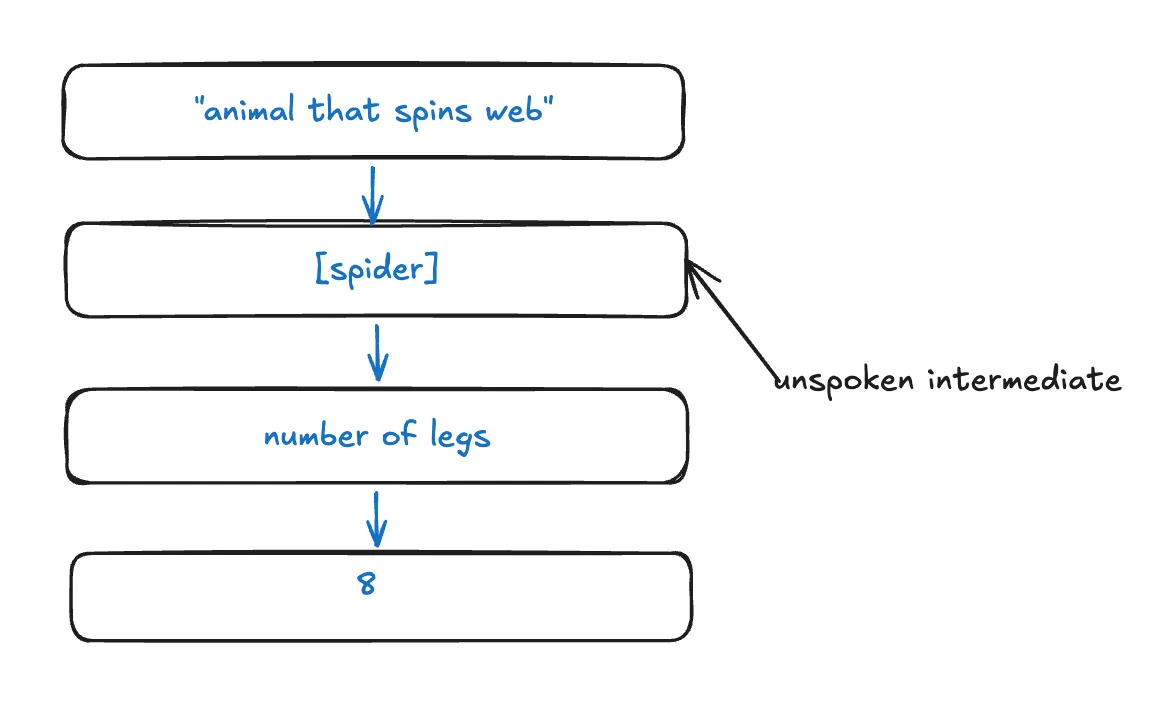
Unspoken inference from “animal that spins webs” through an illustrative spider concept to the answer 8.

the prompt never says spider. the output is just 8.

so the question is simple: can we detect the unspoken spider step, and show that the model actually uses it?

the paper does both. it finds a spider-associated direction inside the residual stream, then swaps its coordinates for ant. the answer flips from 8 legs to 6. across 50 two-hop questions, this kind of swap succeeds in 54% of trials on Haiku 4.5 and 70% on both Sonnet 4.5 and Opus 4.5. a possible cheat would be that the spider direction already contains a bit of 8, so swapping spider for ant is secretly swapping 8 for 6. they check this by swapping the answers themselves instead of the unspoken intermediates; the intermediate swap is what actually moves the conclusion. that experiment is here in the paper.

that is the whole vibe of the paper. not just “we can see a word”, but “this representation was actually being used”.

two things the paper introduces

ok. two objects.

the J-lens is the microscope. it finds verbalizable directions.
the J-space is the sparse set of activation states you can build from those directions.

the workflow is basically:

residual stream → Jacobian lens → J-lens vectors → sparse J-space → read + write + workspace tests

they are not claiming that a transformer recreates the brain’s full global workspace architecture, or that these experiments settle whether a model has subjective experience.

where these representations live

every transformer model has a residual-stream vector. you can learn about the residual stream from this paper.

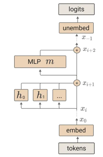
tokens go in, get embedded, sit in a residual stream, and get unembedded into logits.

the vector is called $h_\ell$ . if we think vaguely it is just thousands of numbers, but we want to know “what concept is the vector carrying right now”.

layers keep rewriting that same vector. by the last layer it is in a format the unembedding $W_U$ can turn into next-token scores. in the middle it is messier. that middle is the interesting part.

why the logit lens is not enough

the J-lens is basically a more justified, improved version of the logit lens.

what logit lens does is take a hidden state, say $h_\ell$ , ignore the other layers, and simply do $W_U h_\ell$ . it decodes the middle of the network with the final output decoder.

\operatorname{logit\text{-}lens}(h_\ell) = W_U h_\ell

j-lens puts one extra map in the middle, $J_\ell$ , which stands for “how this layer usually turns into the final layer”:

\operatorname{j\text{-}lens}(h_\ell) = W_U J_\ell h_\ell

that is like reading an unfinished engineering drawing with a legend intended for the finished drawing. the later layers still have work to do. the coordinate system is not finished yet.

residual connections make this less wrong near the end of the model. that is why logit lens often looks fine in late layers and garbage earlier.

the jacobian as a local microscope

jacobian lens fixes this by adding $J_\ell$ . it approximates the remaining network.

suppose the rest of the model after layer $\ell$ is just some function:

h_L = F_\ell(h_\ell)

if we nudge the current activation a tiny bit:

h_\ell \rightarrow h_\ell + \Delta h

then locally:

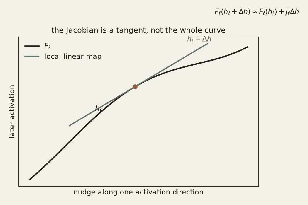
F_\ell(h_\ell + \Delta h) \approx F_\ell(h_\ell) + J_\ell \Delta h

A nonlinear curve with a tangent line at the current activation, showing that the Jacobian only matches nearby changes.

notice: both the direction and size of the resulting change in the final hidden state.

here $J_\ell$ is standing in for the local jacobian of this one activation. the true tangent is prompt-specific. later they average those jacobians into one map per layer. that average is what people mean by the j-lens $J_\ell$ .

the Jacobian captures the model’s local sensitivity around the current activation, not the exact global transformation of the whole network.

the change cannot be too big. the jacobian only accounts for small perturbations, so the linear approximation can break down.

we are doing a linear APPROXIMATION. there are many nonlinear functions after layer $\ell$ in a transformer. $J_\ell$ is a tangent, not the whole remaining network.

building the j-lens

so the simplified j-lens is $W_U J_\ell h_\ell$ . that is the important correction. $W_U h_\ell$ was logit lens. j-lens puts $J_\ell$ in the middle.

they do not use the jacobian of one prompt. the jacobian is averaged across

different prompts
different source token positions
different future output positions

J_\ell = \mathbb{E}_{t,\, t'\ge t,\, \text{prompt}} \left[ \frac{\partial h_{L,t'}}{\partial h_{\ell,t}} \right]

averaging removes a lot of prompt-specific noise and gives a more general layer-level map: across many contexts, which changes at layer $\ell$ tend to make which future words easier to say?

also, dimension-wise: since $h_\ell, h_L \in \mathbb{R}^d$ , each $J_\ell$ is simply a $d \times d$ matrix (e.g. $4096 \times 4096$ ). because it is precomputed and averaged offline once per layer, running the J-lens during inference doesn’t require backprop or recomputing Jacobians, so it is just one fast matrix-vector multiplication $J_\ell h_\ell$ .

then the complete readout is:

\operatorname{lens}(h_\ell) = \operatorname{softmax}\!\left( W_U \operatorname{norm}(J_\ell h_\ell) \right)

each vocabulary token $t$ gets a direction $v_t$ from that map. think of $v_t$ as “the way $h_\ell$ should point if the model is poised to say $t$ later.”

the flow is like this:

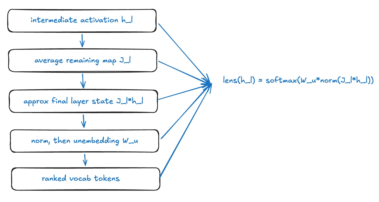
Sequential J-lens pipeline from an intermediate activation through the averaged Jacobian, normalization, unembedding, softmax, and finally ranked tokens.

in code that is just:

def j_lens(h_ell, J_ell, W_U, norm, softmax):
    return softmax(W_U @ norm(J_ell @ h_ell))

$J_\ell$ is not some extra network they trained to make hidden states prettier. it comes from the model itself: how does changing the intermediate state affect the eventual final state?

$v_{\text{spider}}$ does not literally mean the model is internally writing the english word “spider”. it means the activation contains that token’s direction. typical causal effect: the model is more ready to say spider later.

one real limit: the basic j-lens only sees concepts that fit in a single vocab token. spider is easy. multi-token stuff is messier.

reading and writing activations

once you have those directions you can read them or write them.

reading

three versions of reading:

full vocabulary readout. run the softmax above, look at the top tokens. this is the usual “what words appear in the lens?”
single-concept probe. for one token $t$ you just look at $\langle v_t, h_\ell \rangle$ . big value means the current activation is aligned with the model’s general “say something like $t$ later” direction.
sparse decomposition. do not ask “which individual vectors have high similarity?”. ask “what small set of vectors together reconstruct this activation?”

writing

instead of only observing concept directions, we can deliberately modify them.

simplest write is steering:

h \leftarrow h + \alpha v_t

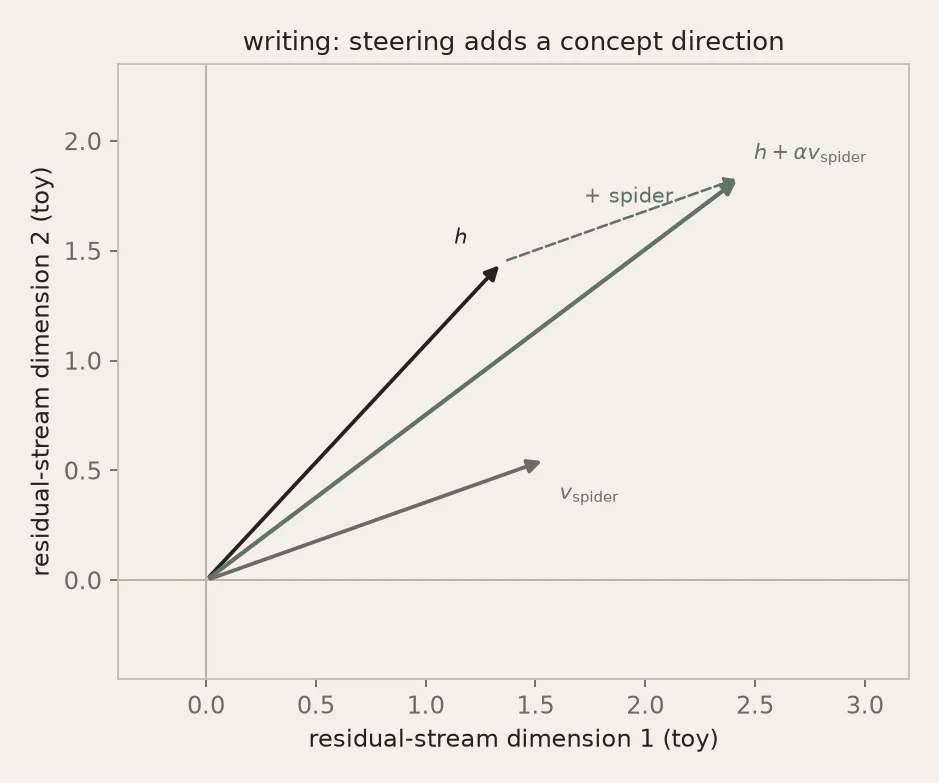
suppose $t = \text{spider}$ . then $h' = h + \alpha v_{\text{spider}}$ .

Steering adds a spider-associated direction onto the current residual-stream vector.

ablation is the opposite. project that component out, or steer with negative $\alpha$ .

Ablation removes the spider-associated component from the current residual-stream vector.

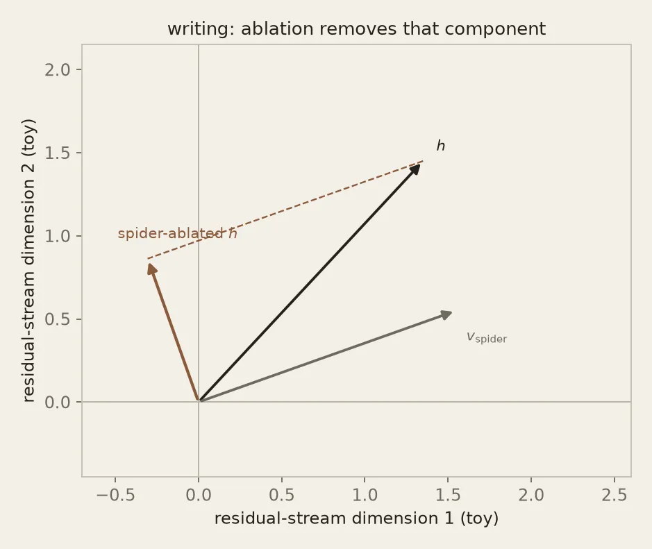
then there is swapping / patching. take the coordinates along $v_{\text{spider}}$ and $v_{\text{ant}}$ , swap them, leave everything orthogonal to those two vectors alone. that is the spider → ant thing. output goes 8 → 6.

so:

reading asks what is in there
writing asks whether that thing is actually being used

from j-lens vectors to j-space

at each layer there is one j-lens direction per vocabulary token:

\{v_1, v_2, \ldots, v_{|V|}\}

the residual vector might be a few thousand dimensions while the vocab is tens or hundreds of thousands of tokens. so these directions are overcomplete. they are not an ordinary orthogonal basis. there is no unique way to write $h_\ell$ as a mix of them.

that overcompleteness does not by itself prove the vectors are semantically similar. it just means the dictionary is too big for a unique decomposition.

separately, a lot of those vectors really do point the same way. spider / arachnid / spiders.

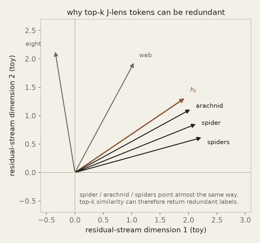
Toy residual-stream plot where spider, arachnid, and spiders point almost the same way, so a top-k list repeats one concept.

notice:

spider
arachnid
spiders

all point in almost the same direction.

suppose $h_\ell$ points toward that region. then all three inner products can be large. say:

spider     0.94
arachnid   0.91
spiders    0.89

softmax is just the usual thing. you have a vector of scores (the logits after $W_U \operatorname{norm}(J_\ell h_\ell)$ ). softmax turns them into a probability distribution:

p_i = \frac{e^{z_i}}{\sum_j e^{z_j}}

bigger logit, bigger probability, they all sum to 1. then you sort.

if you simply choose the top 3, you would conclude:

active concepts:
spider
arachnid
spiders

but that’s arguably one underlying concept showing up three times.

so j-lens vectors are non-orthogonal. they overlap. top-k on the softmax is still a useful readout. it just is a redundant inventory.

top-k is not useless. it is how you read the lens. sparse nonnegative decomposition is what you use when you want a less redundant list of active concepts.

that changes the question from “which individual vectors have high similarity” to “what small set of vectors together”. typically:

h_J \approx \sum_{i=1}^{k} a_i v_i, \qquad a_i \ge 0, \qquad k \le 25

that mix is the j-space component. whatever is left is outside j-space.

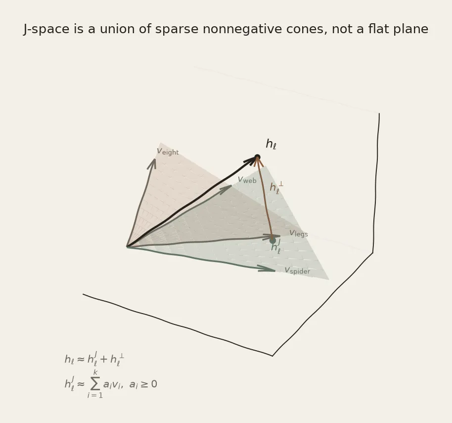
Three-dimensional sketch of J-space as a union of sparse nonnegative cones, with the nearest J-space component of an activation and the leftover component marked.

for a fixed $k$ , j-space is a union of sparse nonnegative cones. one cone for each choice of $k$ vectors. it is not a flat linear subspace. the leftover $h_\ell^\perp$ can be most of the vector. in the paper the j-space part is usually a small slice of variance. the claim is not “most of $h_\ell$ is workspace”. the claim is that this small part is the privileged part.

does j-space behave like a workspace?

these 5 tests are about a subset of the residual stream, not the full residual space. we can’t really say it is the workspace. we can just poke it and see if it behaves like one. the experiments live in the paper.

verbal report

if a concept is in the active workspace, asking “what are you thinking about?” should let the model name it.

sonnet is told to think of a sport, then say it. Soccer shows up in the late j-lens, and it says soccer. swap soccer for rugby inside the model and the spoken answer becomes rugby. they repeat this across fourteen categories. the implanted word tends to move toward the top of the output, not always into first place.

late layers are already near the output though, so that one is a bit cheap. the cooler version plants the concept earlier in the user turn. later, when you ask it to introspect, it reports the planted thing. it does not spam the word the whole time.

directed modulation

can i tell the model to keep something in mind, and does that concept appear internally even if it is not saying it?

example: concentrate on citrus fruits while copying “The old painting hung crookedly on the wall.” around ook in crookedly, the output is still just the sentence. the j-lens is sitting there with orange, lemon, fruit, thinking, focused.

another version silently does $3^2-2$ while copying. the readout goes arithmetic → nine → seven. the copied sentence does not change.

so output ≠ workspace.

“ignore X” still leaves a bit of X in there. like the white bear thing. control exists. it is just not perfect.

internal reasoning

this is the one i care about most.

take $(4+17)\times 2+7$ . the model needs 21, then 42, then 49. those intermediates show up in the lens in that order. if you patch them, the rest of the calculation moves.

same energy as spider. spider is the unspoken middle step. swap it, 8 becomes 6.

70% is not 100%. failed swaps matter. sometimes the concept is weakly loaded. sometimes it is not a single vocab token.

flexible generalization

this one sounds awful in the paper but the idea is really cool.

imagine the concept FRANCE. the model should be able to feed the same representation into capital / language / continent. swap it for CHINA and the same machinery should now give beijing / chinese / asia.

in programmer language, the workspace vector is the argument:

country = France
capital(country)
language(country)
continent(country)

replace country = China without changing the functions.

they tried this across countries, months, animals, number words. 16 functions. 76 of 192 swaps put the target answer on top. crank the swap stronger and it becomes 101 of 192. countries work better than number words. if the source concept was barely there to begin with, the swap is weaker.

so: reuse is real. it is not a perfectly typed variable system.

selectivity

if literally everything inside the model counted as the workspace, the idea would be useless.

take a spanish passage. the model can continue it, notice a french sentence that does not belong, say “this is spanish”, or answer flexible stuff like famous authors and the pre-euro currency. swap spanish → french and the explicit report / flexible answers move. garcía márquez can become victor hugo, hola can become bonjour. continuation and “wait, that sentence is weird” mostly stay put.

boring routine work can live outside j-space. the fancy report-and-reuse stuff leans on it. that is selectivity.

the thing i keep coming back to is small: between raw hidden computation and the final answer, there seems to be a thin verbalizable layer where some intermediate concepts become unusually easy to report, reuse, and intervene on.

the J-lens gives us an imperfect microscope for that layer. the J-space is the sparse geometry it reveals. neither is the whole model, which is probably why the result is interesting.

this was the theory. part 2 will be the implementation/experimentation with qwen models with visual proofs, and part 3 will be a from-scratch (maybe) Jacobian-lens implementation.

i am working on that. peace.